Bayesian Approaches to Variable Selection

Introduction and example demonstration

Kehe Zhang

November 17, 2023

Outline

• Introduction

  • Motivation
  • Traditional variable selection
  • Bayesian Framework

• Bayesian Approach to Variable Selection

  • Model setup
  • Bayesian model selection
  • Spike-and-slab priors
  • Shrinkage priors

• Application and Extensions

  • Example in Nimble
  • Recent Developments

Introduction

Motivation

Big Data Challenge:

• Biology/Genomics/Health Care

• Public Health/Environmental Science

• Economics/Political Science

• Industry/Technology

Given:

• \(Y\), an outcome of interest (AKA response or dependent variable)

• \(X_1\), …, \(X_p\), a set of \(p\) potential explanatory variables (AKA covariates or independent variables).

How can we select the most important variables?

In genomic studies where high-throughput technologies are used to profile thousands of genetic markers, only a few of those markers are expected to be associated with the phenotype or outcome.

Variable selection is especially important in situations where a large number of potential predictors are available.

The inclusion of unnecessary variables in a model has several disadvantages, such as increasing the risk of multicollinearity, insufficient samples to estimate all model parameters, overfitting the current data leading to poor predictive performance on new data and making model interpretation more difficult

Variable Selection

Linear Regression Model

\[ \boldsymbol{y}_{n \times 1} = \boldsymbol{X}_{n \times p} \boldsymbol{\beta}_{p \times 1} + \boldsymbol{\epsilon}_{n \times 1} \]

• \(\mathbf{X}= (\mathbf{x}_1',\ldots, \mathbf{x}_n')'\) is the design matrix of covariates

• \(\boldsymbol{\beta}=(\beta_1, \beta_2, \ldots, \beta_p)'\) denotes a vector of coefficients

• \(\boldsymbol{y}\) is a vector of responses \((y_1, y_2, \ldots, y_n)'\).

• \(\boldsymbol{\epsilon} \sim \mathcal{N}(\boldsymbol{0}, \sigma^2 \boldsymbol{I}_n)\).

Traditional Methods:

• Hypothesis testing methods:

  • Forward/backward, stepwise and best subset selection
  • The OLS estimator: \[ \hat{\beta}_{OLS} = (X'X)^{-1}X'y = \text{arg min}_\beta \ ||y - X\beta||^2\]

• Penalized parameter estimation methods:

  • LASSO, Ridge and Elastic net.
  • The Ridge estimator: \[ \hat{\beta}_{\text{Ridge}} = \text{arg min}_\beta \ ||y - X\beta||^2 + \lambda||\beta||_2 \]
  • The Lasso estimator: \[ \hat{\beta}_{\text{Lasso}} = \text{arg min}_\beta \ ||y - X\beta||^2 + \lambda||\beta||_1 \]
  • Pros:
    • Controlled by a single hyperparameter
    • Scalable to large datasets
    • Well-developed theoretical foundation
  • Cons:
    • Struggles with highly correlated predictors
    • Ignoring uncertainty in the model selection process

• Typical Strategy: sequentially change model until a good fit is produced, and then base inferences/predictions on the final selected model. Strategy is flawed in ignoring uncertainty in the model selection process - leads to major bias in many cases.

• There is typically substantial uncertainty in the model & it is more realistic to suppose that there is a list of a priori plausible models

Bayesian Framework

The Bayesian approaches thus differ from frequentist approach by its ability to incorporating prior information, which plays an important role in variable selection and often serves as a means of stabilizing inferences in high-dimensional settings.

The variable selection can be considered as a special case of model selection problem in which each model under consideration corresponds to a distinct subset of variables.

• Bayesian Inference \[ p(\theta|Y) = \frac{ p(Y|\theta)p(\theta)}{ \int_{\Theta} p(Y|\theta) p(\theta) d\theta } \propto p(Y|\theta)p(\theta) \]

• Incorporate a priori belief of the models and parameter estimates.

• The uncertainty of the model is estimated through the posterior probability of each possible model and the distribution of the posterior parameters.

• The posterior probability provides a more straightforward interpretation of variable importance, and it can be used to compare non-nested models.

• Bayesian linear regression maximum a posterior (MAP) estimator: \[ \hat{\beta}_{\text{MAP}} = \text{arg max}_\beta \ p(\beta|Y) \]

  • With a Laplace (double-exponential) prior \(\rightarrow \hat{\beta}_{\text{Lasso}}\)
  • With a Gaussian prior \(\rightarrow \hat{\beta}_{\text{Ridge}}\)

Bayesian Approach to Variable Selection

The goal of model selection is to identify the most likely underlying model that generates the data.

• In the absence of prior knowledge about which models in the list are more plausible, one often lets \(p(M_\gamma) = 1/M\)

• This penalty is due to the integration across the prior, which is higher in larger models.

• Identifying parsimonious explanation of observed data (post prob concentrates the most parsimonious models that explain the data)

1. Bayesian Model Selection

With \(p\) predictors, we explore \(2^p\) possible models.

Model Representation

• Each model is indexed by a binary vector \(\mathbf{\gamma} = (\gamma_1, \ldots, \gamma_p)\).
  • \(\gamma_j = 1\) implies inclusion of \(X_j\) in the model \(( \beta_j \neq 0 )\), and \(\gamma_j = 0\) implies exclusion of \(X_j\).
  • Example: \(\mathbf{\gamma}= (1, 0, 1, 0, \ldots, 0)\) represents a model with predictors \(X_1\) and \(X_3\) only.
• Let \(\mathcal{M}\) be the space of all possible models and \(M_\gamma \in \mathcal{M}\) be the model that includes the \(X_j\) with \(\gamma_j=1\).
• Prior distributions: \(p(M_\gamma)\) for each model and \(p(\boldsymbol{\theta}_\gamma | M_\gamma)\) for the parameters under each model.
• The posterior probability of a model is given by:

\[ \color{red}{p(M_\gamma| \mathbf{y})} = \frac{\color{steelblue}{p(\mathbf{y}| M_\gamma)} \color{orange}{p(M_\gamma)}}{\sum\limits_{\gamma' \in \mathcal{M}} \color{steelblue}{p(\mathbf{y} | M_\gamma')} \color{orange}{p(M_\gamma)}} \]

• \(\color{steelblue}{p(\mathbf{y}| M_\gamma)}= \int p(\mathbf{y} | M_\gamma, \boldsymbol{\theta}_\gamma) p(\boldsymbol{\theta}_\gamma|M_\gamma) d\boldsymbol{\theta}_\gamma\) is the marginal likelihood of the data for the model \(M_\gamma\) (marginalized over the entire parameter space).

How do we choose among the \(2^P\) models?

• By balancing model fit and model complexity (trade-off): \[\text{Score} = \text{Fit} - \text{Complexity}\]

• Fit: Marginal probability of data given model \(\color{steelblue}{p(\mathbf{y} | M_\gamma)}\)

• Complexity: Prior probability of model \(\color{orange}{p(M_\gamma)}\)

• Unlike the maximized likelihood, the marginal likelihood has an implicit penalty for model complexity.

• The highest posterior probability model (HPM) is then the model with the highest marginal likelihood.

Selection Criteria

Bayes Factor

• One of the most commonly used selection criteria for Bayesian model comparison

• Where ( BF_{12} ) is a ratio of marginal likelihoods of models M1 and M2.

• For each covariate under consideration, PIP is the sum of the normalized posterior probabilities of all models where the covariate is included:

• Bayes factor (BF) can be used to compare and choose between candidate models, where each candidate model corresponds to a hypothesis.

• Unlike frequentist hypothesis testing methods, Bayes factors do not require the models to be nested.

• The BF for model \(M_{1}\) over \(M_2\) is the ratio of posterior to prior odds:

\[ BF_{12} = \frac{p(y | M_1)}{p(y | M_2)} \]

• Interpretation:

  • Values of \(BF_{12} >1\) suggest \(M_1\) is preferred.
  • The larger \(BF_{12}\) is, the stronger the evidence in favor of \(M_1\).

Posterior inclusion probability (PIP)

\[ P(\gamma_j = 1 | y) = \sum_{x_j \in M_\gamma} P(M_\gamma | y) \]

• A higher PIP value for a covariate indicates stronger evidence that it is important for predicting the response variable.

Key Inferences

• Ranking: Order variables by their Posterior Inclusion Probability (PIP).
• Selection: Choose variables with PIP above a certain threshold, e.g., PIP ≥ 0.5.
  • also referred as median probability model (MPM)
• Coefficients: Calculate model-averaged coefficient estimates \(\hat{\beta}\)
• Predictions: Derive model-averaged predictive distributions.
• Correlation: Look at how \(\gamma_p\) is corelated with \(\gamma_q\).

For example, in genomic studies where high-throughput technologies are used to profile thousands of genetic markers, only a few of those markers are expected to be associated with the phenotype or outcome under investigation.

Markov chain Monte Carlo (MCMC)

From computational point of view, when p is small (say p < 20), the size of the model 2p is reasonably small or moderate, exhaustive enumeration of candidate models to compute the Bayes factor or other quantities of interest is possible, and the computation of posterior distribution takes into account all competing models. However, the size of competing models is growing dramatically as p increases, and therefore the exhaustive search of all possible models is not practical when p is large (say p ≥ 20) due to the heavy computational burden. Markov chain Monte Carlo (MCMC) methods are commonly implemented in such cases to perform a stochastic search of model space and allows efficient sampling from the posterior distribution of parameters. The MCMC visits the model space over the iterations and generates the individual posterior model probabilities. The regions of high posterior probability are visited more often than others. Examples of MCMC methods for model selection are the reversible-jump MCMC approach which allows the Markov chain to explore the parameter space of different dimensions [59], Gibbs sampler that is based on pseudo-priors to facilitate the chain jumping between competing models [15].

shrinkage priors that induce sparsity, either by setting the regression coefficients of non-relevant covariates to zero or by shrinking them towards zero, are specified and MCMC techniques are used to sample from the posterior distribution.

• When p is small (P<20), exhaustive search of all candidate models and computation of posterior probabilities is feasible.

• When p is large, MCMC methods are commonly implemented to perform a stochastic search of model space and allows efficient samping from posterior distribution of parameters.

• For example,

  • Reversible-jump MCMC allows the Markov chain to explore the parameter space of different dimensions.
  • Gibbs sampling based on pseudo-priors can facilitate chain jumping between competing models.

Bayesian Approach to Variable Selection

2. Spike and Slab Priors

• The spike-and-slab prior is a two-point mixture distribution on \(\beta_j\): \[\beta_j\sim (1 - \gamma_j)\color{steelblue}{\phi_0(\beta_j)} + \gamma_j\color{orange}{\phi_1(\beta_j)}\]

  • Latent binary indicator \(\gamma_j \sim \text{Bernoulli}(h)\) for \(j = 1, \ldots, p\).
  • \(\color{steelblue}{\phi_0(\beta_j)}\): spike distribution for modeling negligibly small effects.
  • \(\color{orange}{\phi_1(\beta_j)}\): slab distribution for modeling large effects.

• Selecting a subset of important predictors is equivalent to forcing the associated \(\beta_j\) of those non-selected variables to zero.

• Various shrinkage priors have been proposed over the years. A widely used shrinkage prior is the spike- and-slab prior,

• • Allows for jointly selecting the variables and estimating their regression coefficients.

• The discrete spike-and-slab formulation uses a mixture of a point mass at zero and a flat prior (Fig.a), whereas the continuous spike-and-slab prior uses a mixture of two normal distributions (Fig.b). Another widely used formulation puts the spike-and-slab prior on the variance of the regression coefficients.

Stochastic search variable selection (SSVS)

(George & McCulloch, 1993)

• A Popular Spike-and-Slab Approach having an independent normal mixture prior on \(\beta_j\):

\[ \beta_j | \gamma_j \sim (1 - \gamma_j)\mathcal{N}(0, \tau^2_j) + \gamma_j\mathcal{N}(0, c^2_j\tau^2_j) \]

• \(\tau_j\): Small for spike to cluster \(\beta_j\) around zero when \(\gamma_j = 0\).

• \(c_j\): Large for slab to disperse \(\beta_j\) when \(\gamma_j = 1\).

• Facilitates efficient Gibbs sampling for posterior computation:

  • Assign initial values for \(\beta^{(0)}, \sigma^{2(0)}, \gamma^{(0)}\).
  • Sample \(\beta^{(1)}\) from \(f(\beta^{(1)} | y, \gamma^{(0)}, \sigma^{2(0)})\).
  • Sample \(\sigma^{2(1)}\) from \(f(\sigma^{2(1)} | y, \beta^{(1)}, \gamma^{(0)}))\).
  • Sample vector \(\gamma^{(1)}\) componentwise from \(f(\gamma_i^{(1)} | \beta^{(1)},\sigma^{2(1)}, \gamma_{(i)}^{(1)})\).
  • Continue the process until convergence to form a Markov chain - Gibbs sequence.

• The densities of the spike and slab intersect at points \(\pm \xi_j\), \(\xi_j = \tau_j \sqrt{2 \log(c_j) \frac{c_j^2}{c_j^2 - 1}}\), serving as practical significance thresholds for \(\beta_j\).

• With this prior, we have 𝛽 j ∼ N(0,𝜏2 j ), if 𝛾 j = 0, and 𝛽 j ∼ N(0, c2 j𝜏2 j ), if 𝛾 j = 1. The idea here is to set 𝜏 j(> 0) very small, such that those 𝛽 j for which 𝛾 j = 0 will tend to be clustered around 0, and to set cj very large, such that for those 𝛽 j for which 𝛾 j = 1 will tend to be dispersed. The implementation of the normal distributions on the two-points mixture facilitates the efficient Gibbs sampling process for the posterior

• C_i can also be interpretated as the signal to noise ratio at 0.

Bayesian Approach to Variable Selection

3. Continuous Shrinkage Priors

• Idea: place a prior on the coefficients \(\boldsymbol{\beta}\) that concentrates near zero

• Mimics the spike-and-slab prior by a single continuous density.

• LASSO-type priors: Lasso, Ridge, Laplace (Bayes Lasso), Student-t

• Appealing computationally & philosophically to relax assumption of exact zeros

• The Bayesian lasso specifies conditional Laplace priors on \(\beta_j|\sigma^2\), formulated as a scale mixture of normal distributions with an exponential mixing density for the scale parameter. The exponential mixing distribution has a single hyperparameter, which limits its flexibility in differentially shrinking small and large effects. This limitation can be overcome by using a class of shrinkage priors that introduce two shrinkage priors

• The horseshoe prior is flat, introduce two shrinkage parameters, which respectively control the global sparsity and the amount of shrinkage for each regression coefficient. The resulting marginalized priors for βj are characterized by a tight peak around zero that shrinks small coefficients to zero, and heavy tails that prevent excessive shrinkage of large coefficients.

• Laplacian: fat tails; horseshoe prior: singularity of zero (while others have finite density/bounded density near 0), unbounded density near the origin - placing lots of posterior mass near the origin. also fat tails, but really strongly prefers putting betas near zero

• Adaptability: Adjusts naturally to both unknown levels of sparsity and varying signal-to-noise ratios, making it suitable for a wide range of datasets.

• Robustness: It stands strong against large, outlier signals that could otherwise skew results, ensuring the integrity of inferences.

• Good inference algorithms that accommodate this - black box inference algorithms like Hamiltomiom MCMC

• Horseshoe prior:

  • Global-local shrinkage prior: \[\beta_j | \lambda_j, \tau \sim \mathcal{N}(0, \color{orange}{\lambda_j^2}\color{steelblue}{\tau^2)}, \quad \lambda_j \sim \text{Ca}^+(0,1)\]
    • The \(\color{steelblue}{\tau} \rightarrow\) the global shrinkage parameter (i.e. controlling the shrinkage of all coefficients).
    • The \(\color{orange}{\lambda_j} \rightarrow\) local shrinkage parameter (i.e. controlling the shrinkage of a specific coefficient)
    • \(\text{Ca}^+(0,1)\) is a half-Cauchy distribution for the standard deviation \(\lambda_j\).
  • Key advantages: Adaptability and Robustness
  • Hamiltonian MCMC

• Others: Normal-gamma, Dirichlet-Laplace,…

Applications

Implementation in Nimble

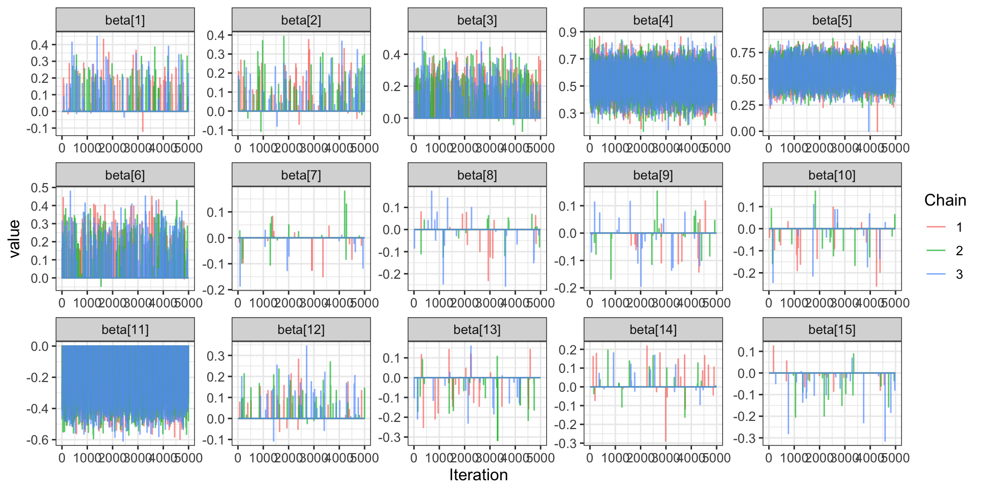
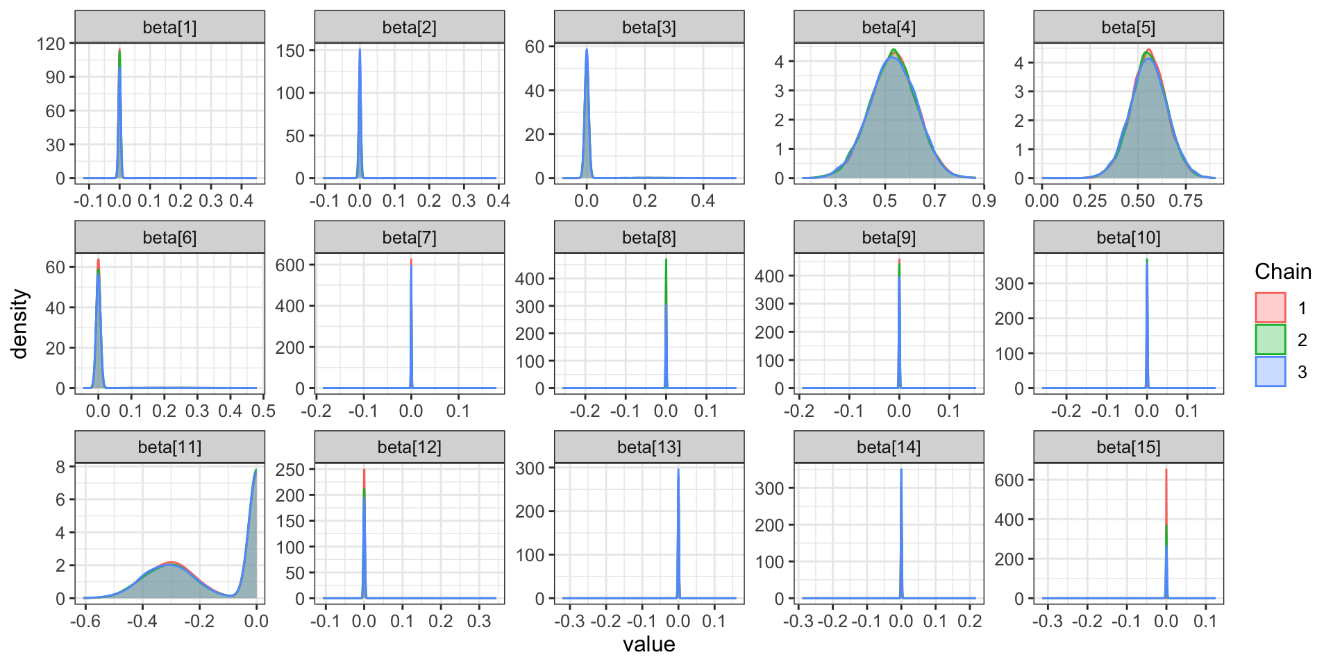
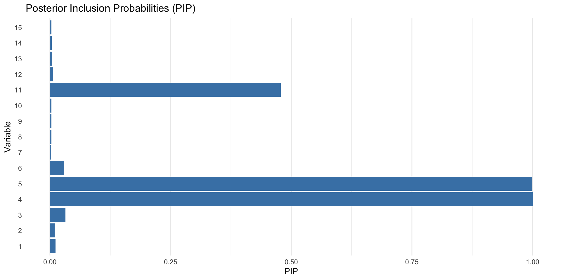
Simulate Data

library(nimble)
library(magrittr)
library(ggplot2)
library(coda)         # for summarizing and plotting of MCMC output and diagnostic tests
library(ggmcmc)       # MCMC diagnostics with ggplot
# data ########################################################################
N <- 100
p <- 15
set.seed(123)
X <- matrix(rnorm(N*p), nrow = N, ncol = p)
true_betas <- c(c(0.1, 0.2, 0.3, 0.4, 0.5),
                rep(0, 10))

y <- rnorm(N, X%*%true_betas, sd = 1)


# standard linear regression ##################################################
summary(lm(y ~ X))

Call:
lm(formula = y ~ X)

Residuals:
     Min       1Q   Median       3Q      Max 
-2.10684 -0.46276 -0.01661  0.46989  2.28986 

Coefficients:
            Estimate Std. Error t value Pr(>|t|)    
(Intercept)  0.08712    0.09133   0.954  0.34292    
X1           0.21730    0.09988   2.176  0.03239 *  
X2           0.13257    0.09221   1.438  0.15423    
X3           0.18998    0.09564   1.986  0.05025 .  
X4           0.59139    0.09006   6.567 4.04e-09 ***
X5           0.55484    0.09385   5.912 7.03e-08 ***
X6           0.20593    0.09652   2.134  0.03579 *  
X7          -0.01480    0.08618  -0.172  0.86407    
X8          -0.03020    0.09241  -0.327  0.74465    
X9          -0.02077    0.08532  -0.243  0.80831    
X10         -0.01368    0.08850  -0.155  0.87750    
X11         -0.29853    0.09007  -3.314  0.00136 ** 
X12          0.10295    0.09271   1.110  0.27000    
X13         -0.09576    0.09896  -0.968  0.33598    
X14          0.05354    0.09192   0.582  0.56180    
X15         -0.03193    0.09359  -0.341  0.73380    
---
Signif. codes:  0 '***' 0.001 '**' 0.01 '*' 0.05 '.' 0.1 ' ' 1

Residual standard error: 0.8465 on 84 degrees of freedom
Multiple R-squared:  0.5672,    Adjusted R-squared:  0.4899 
F-statistic: 7.339 on 15 and 84 DF,  p-value: 4.94e-10

Nimble Code

# linear model with indicator variable ########################################
lmIndicatorCode <- nimbleCode({
  
   # likelihood
  for(i in 1:N) {
    pred.y[i] <- inprod(X[i, 1:p], zbeta[1:p])
    y[i] ~ dnorm(pred.y[i], sd = sigma)
  }
  
   # beta
  for(i in 1:p) {
    z[i] ~ dbern(psi) ## indicator variable for each coefficient
    beta[i] ~ dnorm(0, sd = 10)
    zbeta[i] <- z[i] * beta[i]  ## indicator * beta
  }
  
  # prior
  sigma ~ dunif(0, 20)  ## uniform prior per Gelman (2006)
  psi ~ dunif(0,1)    ## prior on inclusion probability
  
})

## constants ##
lmIndicatorConstants <- list(N = 100, p = 15)

## initial values ##
lmIndicatorInits <- list(sigma = 1, psi = 0.5,
                         beta = rnorm(lmIndicatorConstants$p),
                         z = sample(0:1, lmIndicatorConstants$p, 0.5))
## data ##
lmIndicatorData  <- list(y = y, X = X)

### Define and compile the model
lmIndicatorModel <- nimbleModel(code = lmIndicatorCode, 
                                constants = lmIndicatorConstants,
                                inits = lmIndicatorInits, 
                                data = lmIndicatorData)

### Configuring RJMCMC
lmIndicatorConf <- configureMCMC(lmIndicatorModel)
lmIndicatorConf$addMonitors('z')
configureRJ(lmIndicatorConf,
            targetNodes = 'beta',
            indicatorNodes = 'z',
            control = list(mean = 0, scale = 0.2))

# Check the assigned samplers
lmIndicatorConf$printSamplers(c("z", "beta"))

# Build and run Reversible Jump MCMC
mcmcIndicatorRJ <- buildMCMC(lmIndicatorConf)
cIndicatorModel <- compileNimble(lmIndicatorModel)
CMCMCIndicatorRJ <- compileNimble(mcmcIndicatorRJ, project = lmIndicatorModel)
# Set seed
set.seed(123)

### Run MCMC
system.time(
  samplesIndicator <- runMCMC(CMCMCIndicatorRJ, 
                              niter = 10000, 
                              nburnin = 5000,
                              nchains = 3,
                              summary = TRUE,
                              samplesAsCodaMCMC = TRUE)
)

#save(samplesIndicator, lmIndicatorModel, file = "nimble_example.rdata")

Check Convergence and Posterior Distribution

Beta coefficients and PIP

Posterior summaries of beta coefficients.

Variable	Mean	Median	St.Dev.	95%CI_low	95%CI_upp
beta[1]	0.0020117	0.0000000	0.0212991	0.0000000	0.0000000
beta[2]	0.0017984	0.0000000	0.0194360	0.0000000	0.0000000
beta[3]	0.0071159	0.0000000	0.0429586	0.0000000	0.1540940
beta[4]	0.5308537	0.5324281	0.0935204	0.3483426	0.7119455
beta[5]	0.5565711	0.5562055	0.0939583	0.3646693	0.7433105
beta[6]	0.0065472	0.0000000	0.0399530	0.0000000	0.1252258
beta[7]	0.0000387	0.0000000	0.0043773	0.0000000	0.0000000
beta[8]	-0.0000297	0.0000000	0.0036451	0.0000000	0.0000000
beta[9]	-0.0000394	0.0000000	0.0045983	0.0000000	0.0000000
beta[10]	-0.0001377	0.0000000	0.0056149	0.0000000	0.0000000
beta[11]	-0.1449557	0.0000000	0.1657057	-0.4523247	0.0000000
beta[12]	0.0007470	0.0000000	0.0107174	0.0000000	0.0000000
beta[13]	-0.0003178	0.0000000	0.0081658	0.0000000	0.0000000
beta[14]	0.0001830	0.0000000	0.0062315	0.0000000	0.0000000
beta[15]	-0.0002390	0.0000000	0.0060827	0.0000000	0.0000000

Model Probabilities

Top 5 models with highest posterior probabilities

z[1]	z[2]	z[3]	z[4]	z[5]	z[6]	z[7]	z[8]	z[9]	z[10]	z[11]	z[12]	z[13]	z[14]	z[15]	N	prob
0	0	0	1	1	0	0	0	0	0	0	0	0	0	0	2314	0.4628
0	0	0	1	1	0	0	0	0	0	1	0	0	0	0	2203	0.4406
0	0	1	1	1	0	0	0	0	0	0	0	0	0	0	87	0.0174
0	0	0	1	1	1	0	0	0	0	1	0	0	0	0	63	0.0126
0	0	1	1	1	0	0	0	0	0	1	0	0	0	0	52	0.0104

With 10,000 iterations, only ~0.2% (55/2^15) of the parameters space was searched.

Extensions and Recent Development

Bayesian variable selection methods have been extended to a wide variety of models.

Multivariate Regression Models

• Spike-and-Slab Priors (Brown et al. 1998)
• Multivariate Constructions (Lee et al. 2017)

• Spike-and-Slab Priors: Variables are selected as relevant to either all or none of the response variables.
• Multivariate Constructions: Allow each covariate to be relevant for subsets or individual response variables.
• Generalized Linear Models: Tailoring selection methods to different distributions of the response variable.
• Random Effect Models: Incorporating variable selection in models with random effects.
• Time-Varying Coefficient Models: Capturing dynamics in the relationship between covariates and response over time.
• Mixture Models: For unsupervised clustering, identifying groups within the data.
• Gaussian Graphical Models: Estimating networks and dependencies between variables in single and multiple datasets.

Further Extensions

• Generalized Linear Models and Random Effect Models (Scheipl, Fahrmeir & Kneib, 2012)
• Time-Varying Coefficient Models (Belmonte,Koop & Korobilis, 2013)
• Spatially-Varying Coefficient Models (Reich et al, 2010) (Hu 2021)

Advanced Model Structures

• Mixture Models for unsupervised clustering (Tadesse and Vannucci, 2005)
• Gaussian Graphical Models (Peterson, Stingo, & Vannucci, 2015) (Li & Zhang, 2010)

References

1. O’Hara RB, Sillanpää MJ. A review of Bayesian variable selection methods: what, how and which. Bayesian Analysis. 2009;4(1):85-117. doi:10.1214/09-BA403

2. George EI, McCulloch RE. Approaches for Bayesian Variable Selection. Statistica Sinica. 1997;7(2):339-373.

3. Carlin BP, Chib S. Bayesian Model Choice Via Markov Chain Monte Carlo Methods. Journal of the Royal Statistical Society: Series B (Methodological). 1995;57(3):473-484. doi:10.1111/j.2517-6161.1995.tb02042.x

4. Tang X, Xu X, Ghosh M, Ghosh P. Bayesian Variable Selection and Estimation Based on Global-Local Shrinkage Priors. Sankhya A. 2016;80. doi:10.1007/s13171-017-0118-2

5. García-Donato G, Castellanos ME, Quirós A. Bayesian Variable Selection with Applications in Health Sciences. Mathematics. 2021;9(3):218. doi:10.3390/math9030218

6. Dellaportas P, Forster JJ, Ntzoufras I. On Bayesian model and variable selection using MCMC. Statistics and Computing. 2002;12(1):27-36. doi:10.1023/A:1013164120801

7. Boehm Vock LF, Reich BJ, Fuentes M, Dominici F. Spatial variable selection methods for investigating acute health effects of fine particulate matter components. Biometrics. 2015;71(1):167-177. doi:10.1111/biom.12254

8. Hu G. Spatially varying sparsity in dynamic regression models. Econometrics and Statistics. 2021;17:23-34. doi:10.1016/j.ecosta.2020.08.002

9. Regresssion I, Geweke J. Variable Selection and Model Comparison in Regresssion. Bayesian Statistics. 1995;5.

10. Kuo L, Mallick B. Variable Selection for Regression Models. Sankhyā: The Indian Journal of Statistics, Series B (1960-2002). 1998;60(1):65-81.

11. George EI, McCulloch RE. Variable Selection via Gibbs Sampling. Journal of the American Statistical Association. 1993;88(423):881-889. doi:10.1080/01621459.1993.10476353

Thank you!